Following my two previous posts, here’s a demo showing a model that was trained on a few words. The female voice is coming from the laptop. It listens to any two digits and reads out the sum.
Following my two previous posts, here’s a demo showing a model that was trained on a few words. The female voice is coming from the laptop. It listens to any two digits and reads out the sum.
What’s the Amharic word for “button”? Amharic, Oromiffa or Tigrigna speakers – if you need to translate ICT words, INSA has a useful glossary here (pdf). I’ve put an online version of it at glossary.ainsightful.com.
Some more examples after training on a bigger dataset. Everything else (model size, hyper-parameters, and so forth) have been kept the same. WER stands for Word Error Rate. Samples were taken from the training set, not validation/test.
Truth: የሚ ወጡት ኤምባሲው ውስጥ የሚሰሩ አባላት ና ጥገ ኞቻቸው እንደሆኑ አሜሪካኖቹ አስታውቀ ዋል
Predicted: የሚ ጡት ምባሲ ውስጥ የሚ ሰርአባላት ነው ትገንቻቸው እንዱሙ አሜሊካንቹ አስ ታውዋል
WER: 19
Truth: አስር ሺ ኢትዮጵያዊያ ንም ቤት አልባ ሆኑ
Predicted: አስር ሺ ኢትዮጵያውያ ንም ቤት አልባ ሆኑ
WER: 1
Truth: ያን ያህል ተዳርሰ ን እንወስ ና ለ ን እንጂ ውሳኔ ለ ማግኘት ወደ በላዩ የ ኢትዮጵያ ፉትቦል ፌዴሬሽን አን ሄድ ም
Predicted: የን የህል ተዳርሰንወስና ለን ንጅ ውሳኔለ ማግት ተወደ በላ ይ ኢትዮጵያ ፉት ቦል ፌዴድ ሽን ንደው
WER: 24
Truth: ሰውዬው ሚስቱ ን በጣም እንደሚ ወዳት በ ለ ሆሳ ስ ነገራት
Predicted: ሰውዬው ሚስቱ ን በጣም እንደሚ ወዳት በ ለሆሳስ ነገራት
WER: 2
Truth: በ መከላከያ ሚኒስቴር ሹም ሽር እና እስር እየተካሄደ ነው
Predicted: በመካላኪያሚቴርሹም ሽር ና ስር እየ ተካሄዳ ነው
WER: 11
Truth: ኢህ አ ድግ በ ርእሰ ከተማይቱ አዲስ አባ ሀያ ሰባት ወረዳ ዎች በ እርግጠኝ ነት እንደሚ ያሸንፍ እንደሚ ተማመን ገልፇ ል
Predicted: ያድግ በርሰ ከተማይቶ አዲ በባአያ ሰባቶ ረዳዎች በ ርግተኝነት እንደሚያሸነፍ እንደሚ ተማመንገልፇል
WER: 22
Truth: ለምን ስ እና ንገላታ ቸዋለን የሚ ል አስተያየት ሰንዝ ረዋል
Predicted: ለምንስ ና ንገላታቸዋለን የሚ ላ አ ሰያት ስንዝረዋል
WER: 9
Truth: ግን እሱን ከ ሶስት አመት በፊት ሸ ጬ ዋለሁ
Predicted: ግያ ሱም ከሶስት አመት በፊሸጩነሁ
WER: 11
Truth: አህዛብም ከጥፋት ውሀ በኋላ
Predicted: አህዛብም ከጥፋት ሀ በኋላ
WER: 1
Truth: በዚያች አመትም ስለ ከብቶቻቸው ሁሉ ፋንታ እህልን መገባቸው
Predicted: በዚያች አመትም ስለ ከብቶቻቸው ሁሉ ፈንታ እልን መገባቸው
WER: 2
Research in speech recognition for English and Chinese has shown impressive progress recently. However the only product I found for Amharic was Google’s cloud service. It supports Amharic and works surprisingly well. Nevertheless, it would be wrong to conclude the problem had been solved as we don’t know Google’s methodology and evaluation of it. On top of that, their work is proprietary. There needs to be an open research to speed up progress and make it open for wider use.
This post explains how I applied Deep Recurrent Network to train a speech recognizer for Amharic. I’ll share details of my approach, dataset, and results. Knowledge of Deep Learning and RNNs is beneficial although not necessary. All my work is available on github.
First, it’s helpful to understand what we are up against. Research in speech recognition started way back in the 1950s. Why did it take too long? It turns out there is variation in how we pronounce words which makes recognition tricky. Let’s see an example. Here is a recording of the same speaker saying the same word.
Let us now plot the audio signals. These are basically one dimensional array of numbers. We see the two clips have different signals.
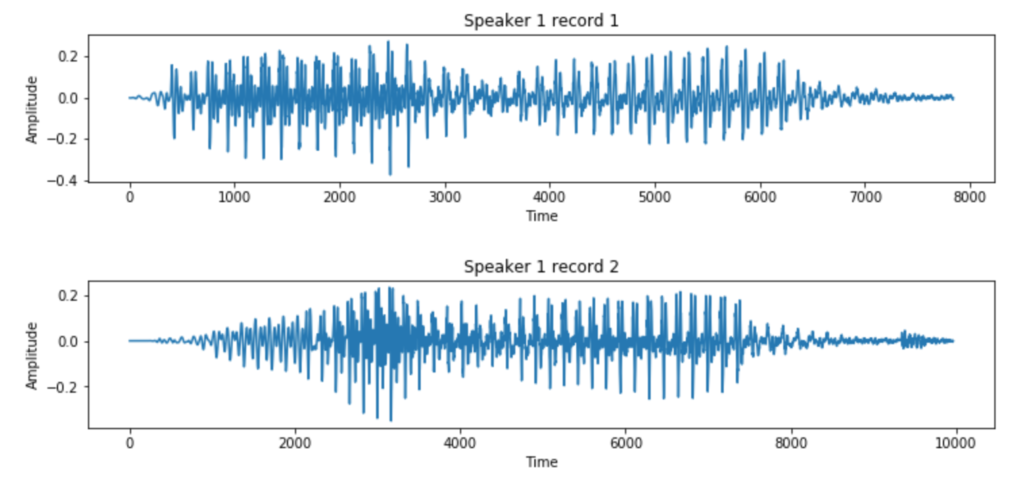
And here is a second speaker, this time female, saying the same word.

The second speaker’s recording looks even different from that of the first. To make the problem worse, there are different accents, some people speak fast while others a bit more slowly, our pitch varies, there can be background noise, and so forth. If the speaker is viewable, we humans pay attention to mouth movements and gestures to aid the listening process. We also consider context – if we didn’t hear a word very well, we fill in the gap by considering what the speaker said before and after.
Data for Amharic speech recognition is extremely difficult to come by. There is plenty of audio data in Amharic but very little transcription of it. Luckily, a friend pointed me to Getalp. They prepared about 10k audio clips totalling 20 hours of speech. Each clip is a few seconds long and comes with its transcription. There are a few hundred separate clips for validation purposes as well.
Key to any machine learning method is extracting features from data. Features represent data and serve as input to the learner. Speech recognition methods derive features from audio, such as Spectrogram or Mel Frequency Cepstrum (MFCC). Audio is split into small blocks, such as 10 milliseconds, and each block is broken into its constituent frequencies. A good example is musical chords. Listen to the following audio.
Three notes are played separately and then all three are played simultaneously. The last piece of sound, called a chord, is similar to what we hear in speech.
I chose to use MFCC over Spectrogram because it produces fewer number of features. Spectrogram can work even better than MFCC as it gives more features. The downside is it needs more data and longer time to train. What does MFCC look like? Let’s take a few seconds of audio clip and plot it’s MFCC features. The result is shown below. Time is on the Y axis. Each horizontal line represents a short audio clip of 10 ms duration. The 13 columns (0-12) represent what’s known as MFCC coefficients in signal processing. Here we simply refer to them as MFCC features. Colors are intensities. Since I chose to use 13 coefficients, each 10ms audio is represented by an array of 13 numbers.
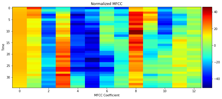
You can read further on MFCC and the reason for choosing 13. I suggest you don’t spend much time on though, because Deep Learning researchers are interested in having the network learn features by itself instead of spending time researching on how to pre-process data for it.
The strength of neural network based solutions lies in the fact that they can be used as generic learning methods to any problem. It has been proven by their application to self driving cars, image recognition, healthcare, and machine translation to name a few. I used Deep Learning (DL) and Recurrent Neural Networks (RNN) because it has shown excellent results and tech companies including Google, Amazon and Baidu use DL for speech recognition.
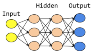
The core idea is to have a network of interconnected nodes (also known as Neural Networks) where each node computes a a function and passes information to the nodes next to it. Every node computes it’s output using the function it was configured to use, and some parameters. The process of learning updates these parameters. The function itself will not change. Initially the parameters are randomly initialized. Then training data is passed through the network, making small improvements to the parameters on every step.
If it all looks like magic, you are not alone! In fact, even leading researchers in the field experiment with different functions and network layouts to see which one works best. There are some well understood functions and network architectures. In case of speech recognition, Recurrent Neural Network (RNN) are used as their output depends not just on the current set of inputs, but on previous inputs too. It’s crucial in speech recognition because predicting what has been said at a particular window of time becomes much easier if what has been said before is known. If you need learning material, there are excellent Machine Learning and Deep Learning courses on Coursera.
Earlier we saw how audio files are broken down into 10 ms chunks and each block represented by an array of features. We then feed each chunk to the network one by one and the network would predict, sometimes called emit, letters. There’s one problem though. When we speak, we don’t say out letters in fixed time durations. Letters are stretched in time as the image below shows.

We solve it by Connectionist Temporal Classification (CTC). In CTC, all the መ’s shown in the image above would be collapsed into a single character, and similarly for “ሄ” and “ድ” characters. What if the word spoken was “መመከር” and we don’t want to collapse the two መ’s into a single “መ”, which would give the wrong prediction “መከር”? For this, CTC introduces a special blank character. Let’s call it B for short. If the network thinks another character was spoken, whether it’s the previous character repeated or a different one, then it emits B. It’s distinct from the space character which is emitted if there is a long silence, normally heard between words. All in all, the network predicts all Amharic characters in the training transcription, B and space.
What we really get during prediction is probabilities for each character. So we end up with a matrix showing probabilities for each character on each time step. Let’s see an example. Listen to the following clip.
I will go into detail about how I built the machine learning model itself. For now though, take a look at the predicted probabilities. Since the full prediction matrix is too big, I have removed predictions for most of the characters except the interesting ones and removed all time steps except the ones most relevant to the first word.
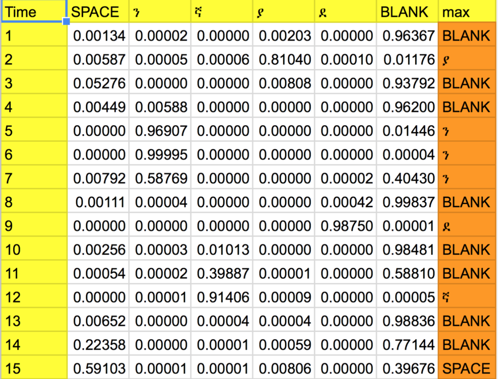
In the max column we simply take the character with the maximum probability in each time step (row). It’s called a greedy approach.
Although greedy approach worked just fine in our particular example, it’s not the ideal solution. For example “ያያB”, “ያBB”and”BያB” are three paths which all result in the same prediction “ያ” after collapsing. So what we really need is to find a more holistic probability which considers all the paths that would lead to the same transcription. For example, for the first time step if “ላ” turned out to have the highest probability, a greedy approach will simply pick “ላ” without comparing the overall probability of all paths that start with “ላ” with those that start with “ያ”.
The ideal solution would take the entire sequence of characters that could ever be predicted in the duration of the clip. Then for each it would find all the paths that lead to that particular sequence of characters. Finally, the probabilities for each paths are summed up. The result would be probabilities for each sequence of characters in the entire time step. We then simply pick up the character sequence with the maximum probability. This operation has exponential complexity. There are 224 characters in my setup. Let’s take a 5 second clip and assume we split each second into 100. We’re end up with 224^500 paths to process! It’s not feasible at all. So we do a beam search. Instead of considering all characters, we remove the ones that have too little probability to be considered. We also look ahead in shorter time steps instead of the entire clip.
To sum up, CTC allows us to take probabilities from the network and decode them into a sequence of characters.
We have pre-processed audio signals to get MFCC features, and worked out how network predictions can be decoded into letters. Now let’s see what happens in the middle. We need to associate audio signals, represented by MFCC features, with Amharic characters. This part is known as acoustic modelling.
The first model I tried had one RNN layer with Gated Recurrent Unit (GRU) followed by normalization. Finally, there’s a softmax layer to output letter probabilities.
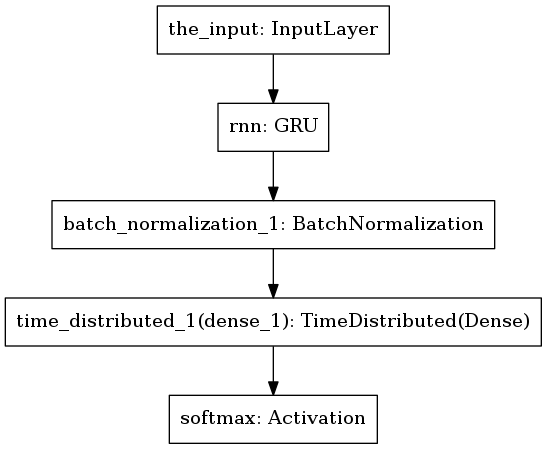
Predicted text was nowhere close to the truth. Here is a typical example.
Truth: ያንደኛ ደረጃ ትምህርታቸው ን ጐንደር ተ ም ረዋል
Predicted: ጌጭሹጭካጌካጐጭቋጭካቋካሶካዤካጪኰጪዊኰጪዊሩሸሩሸቋጪቋጌቼኮጼዛሙጪኰጣኰእኰላጼላጼኰጪህችህጪኰጪኰኩጼጪጧጽቀአእሸሄኬሄአሩህሄህጽጪሹጪሹጪዊአምአ’ዊሸሹራዊዚኙኩጯኩኬጃሹካጪካዊኰአዋኰሹይካጪኰጪሄሙኋሙኛጼጪኰጪኰጪኰጪቆቮሙ’አላሊላሊአሙአሙአሙሩዊዤካዤካቿዊፉዊዋዊዚኩጼዚዋሹአሹዋሙዋሙዋሹአቋዤኬሄርሸሩሸ’ሸቋጃቋጭቋጭጪጭቋካቋሄጭቋጭቋጭ
In the second model I took inspiration from Baidu’s Deep Speech research. One of their improved architecture is Deep Speech 2. Although I haven’t exactly replicated their network, my aim was to have a network a bit similar to theirs. I put a convolutional layer followed by several GRU layers.
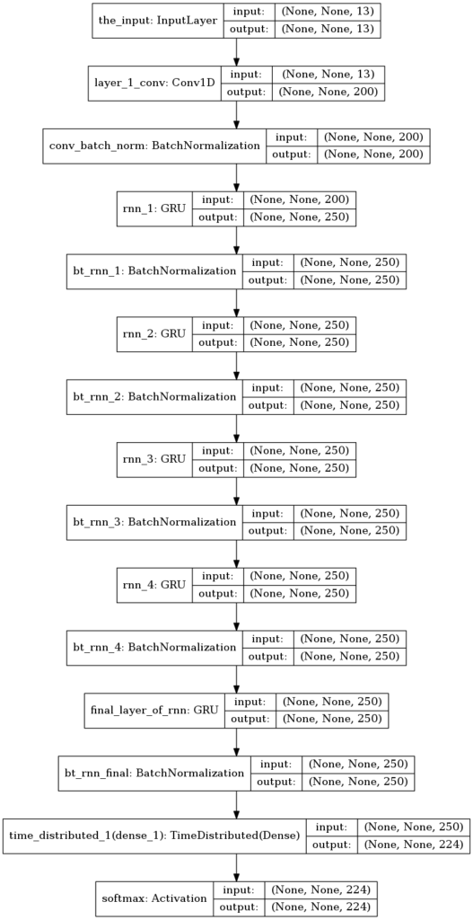
Due to the size of the network, I used GPU instances on Amazon AWS for faster experimentation then ended up running the final training on my laptop. My hardware was Intel i7 8 core CPU. Training consumed about 5 cores and took 3 days to do 40 epochs (rounds) through the data. Investing on GPU would be more appropriate although I feel there are other high priority tasks as I will discuss under Improvements section. Here is how the training history turned out.
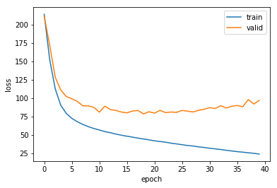
Since validation error increased from epoch 20 onwards, I recorded the model on epoch 22 and evaluated the predictions. Performance on training data was encouraging. Here are two examples.
Truth: ያንደኛ ደረጃ ትምህርታቸው ን ጐንደር ተ ም ረዋል
Predicted: ያንደኛ ደጃት ምርታቸው ቆንዳር ተምረዋል
Truth: ወሬው ን ወሬ ያደረጉ ምስጢረ ኞች ናቸው
Predicted: ወሬ ውድ ወሬ ያደጉ ምስጥረኞች ናቸው
Here is another example, this time on validation data (data not seen by the model before).
Truth: በ ብዛት ግን በ የ መንገዱ ዳር በ የ በረንዳ ው ላይ ም ለ ማደር በ መከልከላቸው ማይ ሀብ ሀብ የተባለ የ ከተማው ቆሻሻ ማጠራቀሚያ ቦታ የሚያድሩ መሆኑን ገልጠዋል
Predicted: ስክእ ብዛት ብንበ የ መንዱዳር በ የ በረን እና ላይን ን ብለ ማደር በ መከል ካ ላቸው ማ ራ ሀ በተባለከት ማቆሻሽ መተረቀ መያበጣ የሚ ያጡ መሆኑ ን ጋልተዋል
It’s far from perfect but it has achieved one of the first steps in machine learning, which is to have a model capable of fitting training data. Word Error Rate (WER) is one way of evaluating speech recognition models. You can find my analysis of that on github as well.
To summarize, here is the full picture of my approach.
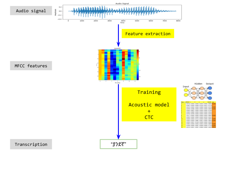
Going forward, there are several interesting venues to build up on. Let me list a few in order of priority.
1. Data
3k hours of speech used to be considered sufficient for training. Big tech companies now use up to 100k hours and beefy hardware. Only 20 hours of data is available for Amharic. More data is needed with different speakers and text. Data can also be synthesized. For example an audio can be duplicated and background noise added on the duplicated data. It helps the model become robust on audio with noise.
2. Language Model
State of the art systems use DL together with a Language Model (LM). Wouldn’t it be nice to take the predicted text and pass it through a spell correction tool? LMs go even further. Let’s say the network is confused between “ተስፋ አለው” and “ተስፋ አለሁ”. It can well decide to predict “ተስፋ አለሁ” if it has the highest probability. A LM would be trained separately on Amharic corpus and no speech is involved. It will know that “ተስፋ አለው” is more probable than “ተስፋ አለሁ”. As opposed to a spell corrector which works after a bunch of words have been written, LM in speech recognition would have a tighter integration with the network. The network would predict probabilities based on speech, and the LM would help predict words. If you think about it, humans do something similar to hear speech as well. Ideally we wouldn’t use LM at all and the network would predict the most likely sequence of words by itself. This is called end-to-end learning and the final goal of deep learning researchers is to get to a point where no pre and post processing is required. The idea is to have the network do pre-processing using it’s initial layers and post processing using the final layers. Doing so requires much larger training data because we would be training the model not only as to how to translate speech utterances into characters, but also how people normally fit words together in that language. So it’s easier to train on textual data separately and then use trained LM model to aid the acoustic model.
3. Model
We have proved to ourselves that the model is capable of fitting training data given to it. The next step is to look into regularization to have a good validation accuracy. This problem can benefit from having more data as well. Different network architectures can be investigated too.
4. Features
As mentioned under Language Model, the goal is to have end-to-end training. And so we wouldn’t even need any pre-processing. Baidu 2 goes a step in this direction by using spectrogram features. There is also some research on using audio signals (the raw data) although it’s still in its infancy.
I had a quick play with Mozilla’s DeepSpeech. It’s a speech recognition engine written in Tensorflow and based on Baidu’s influential paper on speech recognition: Deep Speech: Scaling up end-to-end speech recognition.
The first test it on an easy audio. Recognition was excellent.
➜  deepspeech models/output_graph.pb OSR_us_000_0060_16k.wav models/alphabet.txt models/lm.binary models/trie
Loading model from file models/output_graph.pb
2018-03-18 12:29:45.199308: I tensorflow/core/platform/cpu_feature_guard.cc:137] Your CPU supports instructions that this TensorFlow binary was not compiled to use: AVX2 FMA
Loaded model in 1.470s.
Loading language model from files models/lm.binary models/trie
Loaded language model in 3.867s.
Running inference.
the horse trotted around the field at a brisk pace find the twin who stole the pearl necklace cut the cord that binds the box tightly the red tape bound the smuggled food look in the corner to find the tan shirt the cold drizzle will help the bond drive nine men were hired to dig the ruins the junkyard had a moldy smell the flint sputtered and lit a pine torch soak the cloth and round the sharp or odor
Inference took 85.845s for 58.258s audio file.
And a harder audio with multiple speakers. This time it performed poorly. Words got concatenated into a long gibberish string as well. Increase your volume because this audio is very faint.
➜ deepspeech models/output_graph.pb spkr0.wav models/alphabet.txt models/lm.binary models/trie
Loading model from file models/output_graph.pb
2018-03-18 12:14:09.931176: I tensorflow/core/platform/cpu_feature_guard.cc:137] Your CPU supports instructions that this TensorFlow binary was not compiled to use: AVX2 FMA
Loaded model in 1.440s.
Loading language model from files models/lm.binary models/trie
Loaded language model in 3.872s.
Running inference.
thsalwilljustdoitofntheirfarersothengsimplewefheraway a lot of these dimensions then knew the right way i got something that has all these different masesleavegeenyowothavnoubeewolbeoigisallsortsofviscionsooutmhepolthegoman oundobentyaleininkinoyeihadefferadepraredyshouldbetepridagaitintrytgetdeplenfonhimweresetop for him he roomisitisreallyounderyouoaothinktheyonshidinseholsateayoegoi think we can get pepletocomerethitbutthessasyy osbicsfin volunteer should i pursue that ohdeathetlyyeasotheypay originally they decided not to do go in to the speech soutnutterweerthe'lstillbesoontovolteerf essesfai'comeilityeapeople that are not linguiswereaninaerayaisisabotwerditoelisoreelyeeladersaemlyutbetiio'geeouteadenyersasmeeveeemipunyathealfgethertheothertaetisistecao ng of some sort nowentatatdayihatatjusbefinyge else also atibuelsutorsthegolsandwhatyouknow you can get this and in a gooelyi'lthagotreusedmisstabutyouoappreciateyouknow you can tell him that youll give him a saidhmiytodthe transcripts when they come back koyyitanywaytohvetetransferncesotitiavetoaneiiharesontbletetoconcentabotdoingthebegivingthemtocee immediately because a esissousaiowthispanofstoer aybeofenomegredpornt transfofstageronnanactygivasheelereris owdthostigoboiliketastritflerinhelpotsaton transcoptsreyngphingsyebuteskingsareweninglead out in her a itspeckisityeligotissetingitoyourhonoriagepasigiflgotlios o i ah did bunch of our mivingand still doing a much of our mihingnomin the midst of doing the pefilsforonmin eaven hours to do to copeandit'letayeanotherwordidyoucompettivowel'sidpenstabidsoijustbitasalotodatanedscopedfoinplacinoutofthemovewithanatape ill be done like in about two hours and so a in that for wolbeabltoinworkbymoremeeingssohomrtingofthedodn'tisbothattaisdhatwoncancesonidispreeent eneratingof one alsoanorymonisgeneratingtaclon two hobbies what all soon onsideottewfoaisseplantytososimpllysavedtisyeseeenoheeesilivinganentospiceooknothateodesarethehebilesfombrocesneswhichaeregenneratymone otovethem and for the for a hundred forty hours set and so they they were to degbiesperfileand we had
Inference took 434.213s for 300.000s audio file.
One last difficult one with a single speaker:
➜ deepspeech models/output_graph.pb LDC93S1.wav models/alphabet.txt models/lm.binary models/trie
Loading model from file models/output_graph.pb
2018-03-18 12:06:25.093521: I tensorflow/core/platform/cpu_feature_guard.cc:137] Your CPU supports instructions that this TensorFlow binary was not compiled to use: AVX2 FMA
Loaded model in 1.458s.
Loading language model from files models/lm.binary models/trie
Loaded language model in 4.011s.
Running inference.
she had a ducsuotangresywathorerall year
Inference took 14.435s for 2.925s audio file.
DeepSpeech currently supports 16khz. Other formats can throw the following error:
assert fs == 16000, "Only 16000Hz input WAV files are supported for now!"
Use ffmpeg to convert to 16khz. Example,
ffmpeg -i OSR_us_000_0060_8k.wav -acodec pcm_s16le -ac 1 -ar 16000 OSR_us_000_0060_16k.wav
I used audio files from these sources:
Do you want to document your Play application with Swagger? You may have decided Swagger is the right choice for you but give it a try and you’ll face with poor documentation and issues with different Play versions. This post will go through setting up Swagger for a play application from scratch. If you’d rather cut to the chase and get started with a working setup then you can clone swagger-tutorial and update the sample-swagger project to your needs.
The core of swagger is a specification on how to describe REST API. It specifies how an API should be described using the JSON format. Built around this is Swagger UI that can parse such a specification and provide a good presentation. It also allows for test calls within the UI which is very useful for development.
We will do the following
This post is tested on Play version 2.5.x.
Let’s start off with a working Play application. If you already have a working Play application you can use that and skip to the next section. Bear in mind this post is tested on Play 2.5.x.
If you want to start off with a sample Play project, clone my repo,
git clone git@github.com:tilayealemu/swagger-tutorial
There are two projects.
sample-play: a bare Play appplication
sample-swagger: a Play application with one end point and a swagger doc for it. It has all the changes discussed in this post applied to it.
Build and run the project. You should be able see the root page like so.

Let’s add a simple REST endpoint. We create a “hello” service that takes a name and responds “Hello <name>”
If you cloned the sample-play project add this to the HomeController (if you have your own controller then use that).
def sayHello(name: String) = Action {
  Ok(s"hello $name")
}
Then define the endpoint in your routes file.
GET /hello/:name controllers.HomeController.sayHello(name:String)
Now call the endpoint.

We are now ready to move to Swagger.
Before adding swagger annotation, add this dependency.
libraryDependencies += "io.swagger" %% "swagger-play2" % "1.5.3"
Then go to your controller, such as HomeController, and import some Swagger dependencies.
import io.swagger.annotations.{Api, ApiParam, ApiResponse, ApiResponses}
import play.api.mvc.{Action, Controller}
Annotate the controller class with @Api, and annotate the method too:
@Api
class HomeController extends Controller {

  @ApiResponses(Array(
    new ApiResponse(code = 400, message = "Invalid name supplied"),
    new ApiResponse(code = 404, message = "Name not found")))
  def sayHello(@ApiParam(value = "Name to say hello") name: String) = Action {
    Ok(s"hello $name")
  }
}
Build your code to ensure there are no compilation problems. We can now generate swagger.json that will contain this annotation.
Go to application.conf and add this to enable Swagger
play.modules.enabled += "play.modules.swagger.SwaggerModule"
Then And in routes file add swagger.json. This will list resources in your service.
GET /swagger.json controllers.ApiHelpController.getResources
Then when you access http://localhost:9000/swagger.json you will get the specification for your endpoint.
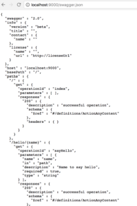
This is the core of what Swagger is. Next up is to use Swagger UI for a pretty view of this specification.
Copy Swagger UI files from the main github repo to your project. You only need the dist directory.
git clone git@github.com:swagger-api/swagger-ui
mkdir swagger-tutorial/sample-play/public/swagger
cp -R swagger-ui/dist/* swagger-tutorial/sample-play/public/swagger
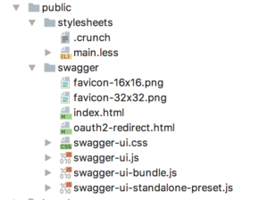
Then update your route file. We will serve swagger under /docs/.
GET        /docs/               controllers.Assets.at(path="/public/swagger",file="index.html")
GET        /docs/*file          controllers.Assets.at(path="/public/swagger",file)
You can go ahead and visit localhost:9000/docs/ but what you will see is a documentation for a sample pet store REST API. Let’s update Swagger UI to use our swagger.json instead. Go to swagger/dist/index.html and change the pet store URL:
url: "http://localhost:9000/swagger.json"
You should now see your service listed.
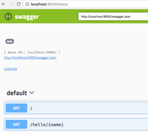
Click on the /hello/{name} endpoint. Click “Try it out”, type a name and click execute. You should get a response and 200 response code.
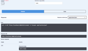
That’s it! You can head over to swagger annotations for more details on annotating services. Remember, if it doesn’t work for you, simply take sample-swagger and change it as you wish.
All comments welcome.
A friend likes sending me puzzles at midnight. It’s called the Emperor’s Proposition and here it is (slightly modified but idea just the same),
You are in prison. The guard can set you free if you win a game. You will be given 100 black marbles, 100 white marbles and 2 bowls. You are allowed to place the marbles in any of the bowls, and you are not allowed to leave any marble outside. Once you are finished, the guard will choose a bowl at random and take out a single marble from it at random. If the marble is black, you win, if its white, you lose. What is the best way of distributing the marbles so you can win?
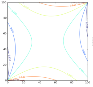
There are many pages with the answer and explanation of the conditional probabilities. Spoiler alert: answer coming up in next sentence. Best choice is to put a single black marble in one bowl and all others in the other. Here is how the probability varies as the composition of marbles is varied. We consider the composition in one of the bowls only because we have just 2 independent variables in this problem.
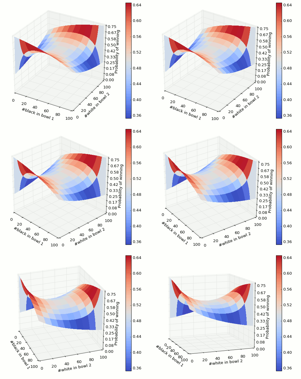
It’s quite a slippery surface 🙂 And contour graph,
Python code,
%matplotlib notebook
from mpl_toolkits.mplot3d import Axes3D
import matplotlib.pyplot as plt
from matplotlib import cm
from matplotlib.ticker import LinearLocator, FormatStrFormatter
import numpy as np

fig = plt.figure()
ax = fig.gca(projection='3d')

def div(a, b):
 return a/np.maximum(b, 1)

# make data
X = np.arange(0.0, 101.0, 1.0)
Y = np.arange(0.0, 101.0, 1.0)
X, Y = np.meshgrid(X, Y)
Z = 0.5*(div(X, (X+Y)) + div((100-X), (200-(X+Y))))

# surface plot
surf = ax.plot_surface(X, Y, Z, cmap=cm.coolwarm,
 linewidth=0, antialiased=False)
ax.set_zlim(0.0, 0.75)
ax.set_zlim3d(0.0, 0.75)
ax.zaxis.set_major_locator(LinearLocator(10))
ax.zaxis.set_major_formatter(FormatStrFormatter('%.02f'))
ax.set_xlabel('#black in bowl 1')
ax.set_ylabel('#white in bowl 2')
ax.set_zlabel('Probability of winning')
fig.colorbar(surf)
plt.show()

# countour plot
plt.figure()
CS = plt.contour(X, Y, Z)
plt.clabel(CS, inline=1, fontsize=10)
CB = plt.colorbar(CS, shrink=0.1, extend='both')
plt.show()
Prime numbers are a lot of fun. One area I think worth considering is to visualise them in different ways to find patterns.
For example mathematicians were recently excited by the finding that the last digit of prime numbers shows some interesting statistical properties. For centuries mathematicians have mulled over prime numbers. It is quite plausible that the next big step would be made by looking at their statistical properties and visualising them in different ways. Since they are stubbornly “random”, the challenge is to find transformations and visualisations that will let us see new patterns which we didn’t know existed. I put random in quotes because although they seem random, the underlying mechanism that generates them is quite precise.
So here are some fun images of them.
To make things easier I downloaded a file with a list of prime numbers this site. There are a total of 78498 primes in the file (or perhaps one less because the file contains number 1, which is not prime).
First the first 100 prime numbers in all their glory,
 2 3 5 7 11 13 17 19 23 29 31 37 41 43 47 53 59 61 67 71 73 79 83
 89  97 101 103 107 109 113 127 131 137 139 149 151 157 163 167
 173 179 181 191 193 197 199 211 223 227 229 233 239 241 251 257
 263 269 271 277 281 283 293 307 311 313 317 331 337 347 349 353
 359 367 373 379 383 389 397 401 409 419 421 431 433 439 443 449
 457 461 463 467 479 487 491 499 503 509 521 523 541
and the last 5 in my file,
999953 999959 999961 999979 999983
Let’s plot the first 100 primes.
Welcome the misbehaving numbers. Let’s plot the difference between successive primes for all primes (remember, around 78 thousand of them). This is known as the prime gap.
The white lines are odd numbers. Since all primes except 2 are odd, the gap between them is always even. Distance between primes seems to be increasing generally but the bottom of the graph remains dark as we progress to the right. It shows that even for large primes, we find primes whose gap is as little as 2. This is actually related to one of the unanswered questions of primes – Are there infinite prime pairs with a gap of 2?
If you find the previous graph too dense here is another one for the first 100 primes.
How about we plot prime gaps as a 2D image? To arrange our 78k primes in more or less square image, we draw the prime gaps row by row, with 280 primes in each row.
There are so many questions we can ask on this plot. For example how frequently are the prime gaps themselves divisible by, say, 23?
row1 ....1....
row2 ...1.1...
....1....
...1.1...
..1.1.1..
Recently ran into the problem of finding the largest image in an html page. This can be useful in page summarisation tasks for example.
Found this scala project which looked promising but failed to compile for me,
https://github.com/GravityLabs/goose
Here is a quick php script that does that.
https://gist.github.com/tilayealemu/2519f54222ad9a7d7ff2b294b2b32a09
Example call,
http://localhost/largest.php?url_without_http=bbc.co.uk

Notes:
In the previous post I talked about Decision Trees. In this post I will talk about how to represent decision trees in SQL.
But first, why would you want to do that? There are Weka (a data mining tool), Scikit Learn (the mainstream machine learning library at the moment), H2O or Spark MLlib (both rooted in big data). However, there are several steps you have to take,
Every step is a hurdle against quick development and deployment. If you have your data in a SQL-like database, wouldn’t it be nice to just have a SQL that expresses a decision tree? If the trained model is a SQL string with no dependencies then steps 3 to 5 are no longer needed.
A popular data for decision tree is the Iris dataset. It was first gathered in 1936 and has since been analysed in numerous research papers. Each row in the dataset represents a sample flower. There are three different species of the Iris flower and all of them are equally represented in the dataset (so there is 50 of each).

Here are the five columns,
What we want to do is learn from the data to give a decision tree that can take the first four columns as input and predict the species name. I wrote a small script that uses scikit to learn a decision tree from this data and translate the decision tree to a SQL.
There are plenty of tutorials on the web about using scikit. So I’ll just point you to my small script that outputs the SQL. It uses scikit to train a decision tree on the 150 rows, takes the decision tree and translates its to SQL. Here is what the result looks like,
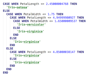
It’s beautiful 🙂 Let’s look at it in detail a bit. The first case shows the Iris Setosa species must have a very distinctive petal length. The second case shows that if petal length is ambiguous then petal width is used to narrow things down.
By the way, the example is not far fetched. An interesting and recent example is how a farmer used machine learning to automatically sort Cucumbers. You can read about it on Google’s blog.
Although NoSQL generated a lot of noise relational databases and SQL still kick ass. We will always deal with tabular data and SQL will remain a powerful language to express database operations. On the other hand, the further our data analysis tool live from our databases, the more mundane work there is to do. Machine learning doesn’t have to be all new technology. A simple SQL query could be just what you need.