Decision trees and SQL (Part 2 – SQL as decision tree)

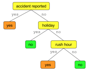
In the previous post I talked about Decision Trees. In this post I will talk about how to represent decision trees in SQL.

But first, why would you want to do that? There are Weka (a data mining tool), Scikit Learn (the mainstream machine learning library at the moment), H2O or Spark MLlib (both rooted in big data). However, there are several steps you have to take,

  1. Feed your data to the library/framework
  2. Train
  3. Persist the model
  4. Figure out the model’s API
  5. Bundle your model with your application together with any dependencies it may have

Every step is a hurdle against quick development and deployment. If you have your data in a SQL-like database, wouldn’t it be nice to just have a SQL that expresses a decision tree? If the trained model is a SQL string with no dependencies then steps 3 to 5 are no longer needed.

An example

A popular data for decision tree is the Iris dataset. It was first gathered in 1936 and has since been analysed in numerous research papers. Each row in the dataset represents a sample flower. There are three different species of the Iris flower and all of them are equally represented in the dataset (so there is 50 of each).

iris

Here are the five columns,

  • SepalLength
  • SepalWidth
  • PetalLength
  • PetalWidth
  • Name

What we want to do is learn from the data to give a decision tree that can take the first four columns as input and predict the species name. I wrote a small script that uses scikit to learn a decision tree from this data and translate the decision tree to a SQL.

There are plenty of tutorials on the web about using scikit. So I’ll just point you to my small script that outputs the SQL. It uses scikit to train a decision tree on the 150 rows, takes the decision tree and translates its to SQL. Here is what the result looks like,

dtsql

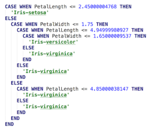
It’s beautiful 🙂 Let’s look at it in detail a bit. The first case shows the Iris Setosa species must have a very distinctive petal length. The second case shows that if petal length is ambiguous then petal width is used to narrow things down.

By the way, the example is not far fetched. An interesting and recent example is how a farmer used machine learning to automatically sort Cucumbers. You can read about it on Google’s blog.

Thoughts on big data

  • If data is huge then a distributed solution becomes necessary.
  • The final output after a lot of churning is still going to be a decision tree, which can be expressed as SQL.
  • SQL can be ran not just on old relational databases, but on new ones too, such as Hive and MemSQL.

Final notes

Although NoSQL generated a lot of noise relational databases and SQL still kick ass. We will always deal with tabular data and SQL will remain a powerful language to express database operations. On the other hand, the further our data analysis tool live from our databases, the more mundane work there is to do. Machine learning doesn’t have to be all new technology. A simple SQL query could be just what you need.

Links

Iris dataset
Demo script
DT in scikit

Decision trees and SQL (Part 1 – Decision trees)

Decision trees and simplicity

Heavy clouds today? Then it will probably rain because we have, many times in the past, seen rain in cloudy conditions. But what if it is cloudy and we are in the middle of summer? Then we can say it is less likely to rain. Every machine learning method has its own approach to modelling how to learn from past data and represent that knowledge.

Decision trees do it in a straightforward way. It’s their simplicity that makes them attractive. Simplicity here is not about finding a mediocre solution in a short time with a vision of applying more complex and better solutions later. It’s about using a good enough method, and it’s about not overcomplicating things too much. A simple model can be all we need.

An example

Suppose we have data with four columns or attributes:

  • Accident reported (true/false)
  • Holiday (date)
  • Rush hour (time)
  • Congestion (true/false)

We try to use the first three attributes to predict the congestion column. Here is an example decision tree that does this. To make use of it, we start by answering the top question: accident reported or not? If an accident is reported we predict there will be congestion. If not, then we are still a bit unsure. So we ask more questions. Our tree is using two other attributes: whether the day is a holiday and whether the time of day is rush hour.


congestion-decision-tree-aisngitht-com

A few more interesting observations:

  • Accidents result in prediction of congestion, irrespective of holiday and rush hour data. This might be wrong. For example an accident on Christmas Day may not result in congestion. But there is nothing stopping us from extending the left branch of the accident node to do some more checks.
  • Our tree considers only three attributes to come to a conclusion. However, other attributes may need to be taken into account for better accuracy. Also, one or more of those being considered here (accident, holiday, rush hour) may have to be removed if it appears that they don’t help much in making predictions any more accurate.

Some interesting questions

How does a decision tree know in what order to put the nodes? For example why not check for rush our before checking for accident? Our tree puts accidents first because it believes accidents are a major factor. A decision tree comes to such conclusions by looking at data. Here is example data that will result in such a conclusion,

  • There was congestion 30% of the time, and
    • 90% of the time – accidents were reported
    • 50% of the time – it was rush hour
    • 1% of the time – it was a holiday

The decision tree algorithm concludes from this data that accidents are the best factor to split the data on. The split results on one big group being split into two smaller groups. The algorithm keeps splitting each group into smaller pieces until each group has a reasonable homogeneity. For example if a certain group is composed of 50% congestion and 50% non-congestion data points then the group must be split further because it is hard to decide who has ‘won’. If a group is composed of 98% congestion and 2% non-congestion, then it can be considered a good split and the whole group is assigned the congestion label.

And how do we know which attributes to use? There are three in our example. How about in other trees? The answer is multifaceted.

  • First of all, we are limited by available data. We stick to what we have or we do some work to obtain data that we think can help improve accuracy.
  • Next, we use domain knowledge. If we have one thousand attributes available to us then using all of them will probably result in a complex tree that doesn’t perform well. For example knowledge of London weather is probably useless for predicting congestion in New York. There is always risk in making such conclusions because data can sometimes show amazing results. On the other hand, we also have risk of overcomplicating our decision tree, also known as overfitting. So we choose the one with less risk, in this case not to include an attribute that we are sure to be irrelevant.
  • Third, a decision tree itself learns which attributes are important. Generally, the less important an attribute is, the lower in the decision tree that it appears. And so pruning the tree translates into leaving out some attributes. To put it another way, we are telling the tree “Checks that appear further down the tree are going into too much in detail. Forget those out and reach to a conclusion earlier”.

Wrap up

That’s pretty much my highlight of decision trees. If you want to delve into technical details a bit more, Chapter 3 of Tom M Mitchell’s Machine Learning book has an excellent explanation of decision trees. For a quick overview see Learning from Data: Decision Trees slides from U Edinburgh.

How can we apply decision trees in a relational database or a database that supports SQL? This will be the topic of my next post.